[1]:

from pathlib import Path
import pandas as pd
from idf_analysis.idf_class import IntensityDurationFrequencyAnalyse
from idf_analysis.definitions import *
from idf_analysis import __version__
print(f'{__version__=}')

__version__='0.2.9'

[2]:

%matplotlib inline
%load_ext autoreload
%autoreload 2

Intensity Duration Frequency Analyse¶

Parameter¶

series_kind:

SERIES.PARTIAL = Partielle Serie (partial duration series, PDS) (peak over threshold, POT)

SERIES.ANNUAL = Jährliche Serie (annual maximum series, AMS)

worksheet:

METHOD.KOSTRA: - DWA-A 531 - KOSTRA - recommented - Parameter formula change at 60 min and 12 h

METHOD.CONVECTIVE_ADVECTIVE: - DWA-A 531 - Unterscheidung in überwiegend konvektiv und advektiv verursachte Starkregen - Parameter formula change at 3 h and 24 h

METHOD.ATV: - ATV-A 121 - Parameter formula change at 3 h and 48 h

extended_durations = Includes the durations steps [0.75d, 1d, 2d, 3d, 4d, 5d, 6d] in the analysis (d=days)

Default duration steps [5m, 10m, 15m, 20m, 30m, 45m, 60m, 1.5h, 3h, 4.5h, 6h, 7.5h, 10h, 12h]

[3]:

idf = IntensityDurationFrequencyAnalyse(series_kind=SERIES.PARTIAL, worksheet=METHOD.KOSTRA, extended_durations=True)

I used the rain-time-series from ehyd.gv.at with the ID 112086 (Graz-Andritz) created with the ehyd-tools package.

You need to install pyarrow or fastparquet to read and write parquet files.

[4]:

data = pd.read_parquet('ehyd_112086.parquet').squeeze('columns')

Get a look at the time-series

[5]:

data.head()

[5]:

datetime
2007-09-17 13:56:00    0.0
2007-09-17 13:57:00    0.0
2007-09-17 13:58:00    0.0
2007-09-17 13:59:00    0.0
2007-09-17 14:00:00    0.0
Name: N-Minutensummen-112086, dtype: float64

[6]:

data.tail()

[6]:

datetime
2019-12-31 23:56:00    0.0
2019-12-31 23:57:00    0.0
2019-12-31 23:58:00    0.0
2019-12-31 23:59:00    0.0
2020-01-01 00:00:00    NaN
Name: N-Minutensummen-112086, dtype: float64

Set the time-series to be used for the calculation of the IDF parameters

[7]:

idf.set_series(data)

define a working directory to save some plots and interim results

[8]:

output_directory = Path('ehyd_112086_idf_data')

create a plot for the interim parameters of the partial series.

[9]:

fig = idf.parameters._interims.plot_series(ncols=7)
fig.set_size_inches(21,12)
fig.set_dpi(60)

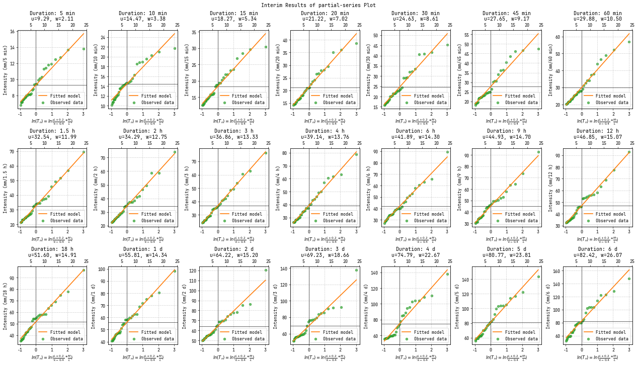
../_images/examples_example_python_api_15_1.png

Intermediate results are created for each new calculation, which are only dependent on the selected series series_kind and the specified/required duration steps. This process takes a few seconds. In addition, these intermediate results contain the parameters required to calculate the rainfall height. The calculation methods and formula-change-durations according to the selected worksheet are already taken into account here.

[10]:

idf.write_parameters(output_directory / 'idf_parameters.yaml')

To save time, it is possible to save the parameters temporarily and when the script is called up again, these parameters are no longer calculated but read from the file.

[11]:

idf.auto_save_parameters(output_directory / 'idf_parameters.yaml')

These interim results can be called up with:

[12]:

idf.parameters.pprint()

{'durations': [5.0,
               10.0,
               15.0,
               20.0,
               30.0,
               45.0,
               60.0,
               90.0,
               120.0,
               180.0,
               240.0,
               360.0,
               540.0,
               720.0,
               1080.0,
               1440.0,
               2880.0,
               4320.0,
               5760.0,
               7200.0,
               8640.0],
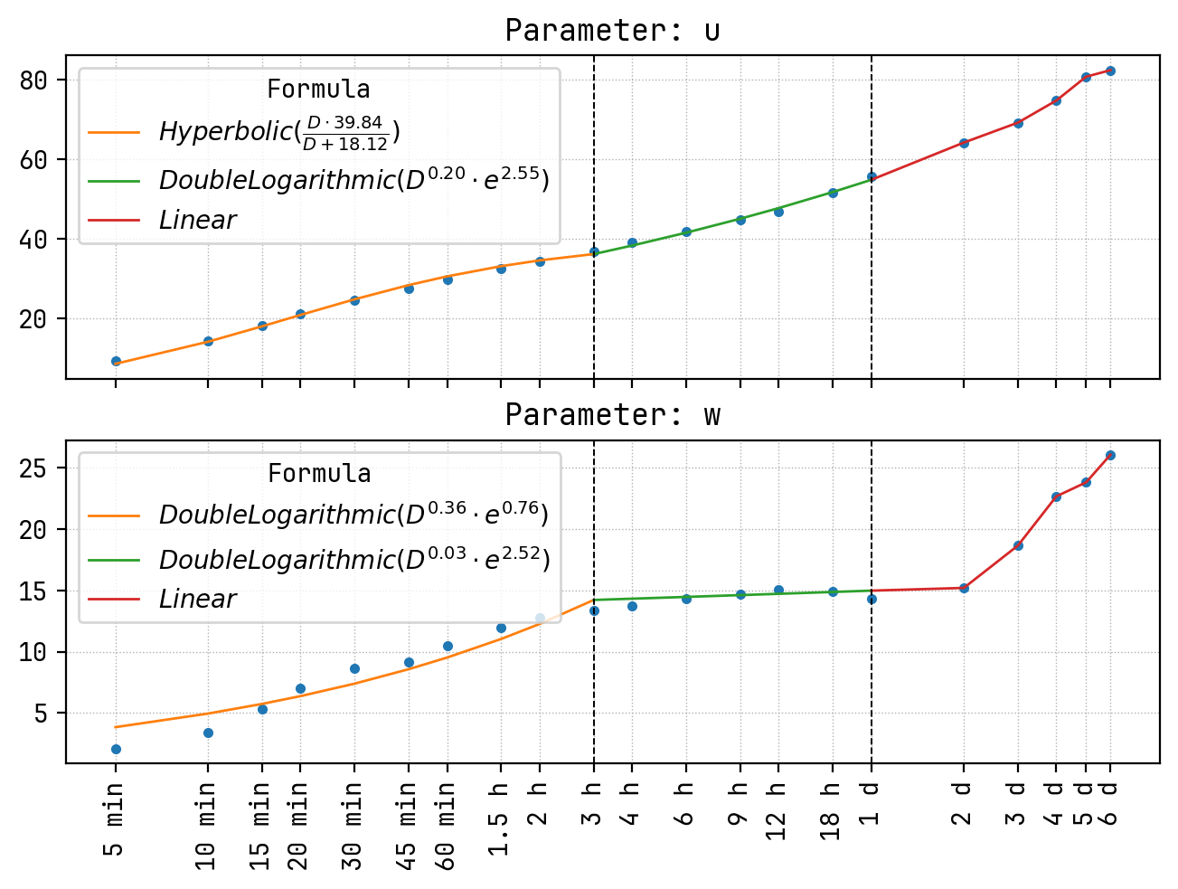
 'parameters_final': {0: {'u': HyperbolicAuto(38.04, 16.10),
                          'w': DoubleLogNormAuto(0.16, 0.55)},
                      60: {'u': DoubleLogNormAuto(2.65, 0.18),
                           'w': DoubleLogNormAuto(1.88, 0.13)},
                      720: {'u': Linear(), 'w': Linear()}},
 'parameters_series': {'u': [9.2852,
                             14.4656,
                             18.2676,
                             21.223,
                             24.6312,
                             27.6473,
                             29.8823,
                             32.5402,
                             34.2917,
                             36.8614,
                             39.1387,
                             41.8902,
                             44.9288,
                             46.8465,
                             51.6007,
                             55.8142,
                             64.2187,
                             69.2324,
                             74.7885,
                             80.7697,
                             82.4165],
                       'w': [2.109,
                             3.3818,
                             5.3372,
                             7.022,
                             8.6112,
                             9.1709,
                             10.5036,
                             11.9877,
                             12.7487,
                             13.3321,
                             13.7618,
                             14.2992,
                             14.698,
                             15.0692,
                             14.9139,
                             14.3355,
                             15.2022,
                             18.6616,
                             22.6725,
                             23.8148,
                             26.0658]},
 'series_kind': 'partial'}

[13]:

idf.parameters

[13]:

<idf_analysis.idf_backend.IdfParameters at 0x321aa8770>

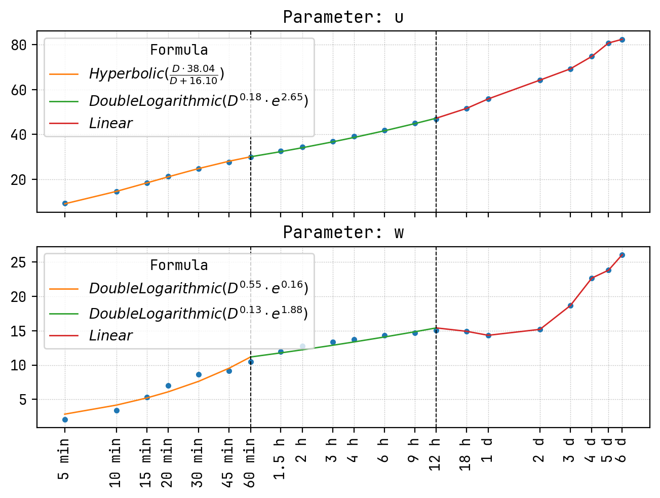
plot the interim results for the final parameters of the function to calculate the rainfall height depending on duration and return periods.

[14]:

fig = idf.parameters.interim_plot_parameters()

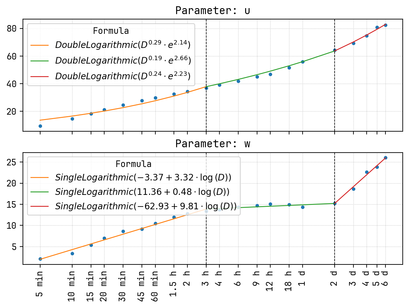
../_images/examples_example_python_api_24_0.png

test also other formulas for the IDF function (According to the older guideline ATV-A 121 (till 2012))

[15]:

idf.parameters.set_parameter_approaches_from_worksheet(METHOD.ATV)
fig = idf.parameters.interim_plot_parameters()

../_images/examples_example_python_api_26_0.png

[16]:

idf.parameters.set_parameter_approaches_from_worksheet(METHOD.CONVECTIVE_ADVECTIVE)
fig = idf.parameters.interim_plot_parameters()

../_images/examples_example_python_api_27_0.png

Calculations¶

[17]:

idf.depth_of_rainfall(duration=15, return_period=1)

[17]:

18.042501067209535

[18]:

print('Resulting rainfall height h_N(T_n={t:0.1f}a, D={d:0.1f}min) = {h:0.2f} mm'
      ''.format(t=1, d=15, h=idf.depth_of_rainfall(15, 1)))

Resulting rainfall height h_N(T_n=1.0a, D=15.0min) = 18.04 mm

[19]:

idf.rain_flow_rate(duration=15, return_period=1)

[19]:

200.47223408010595

[20]:

print('Resulting rainfall flow rate r_N(T_n={t:0.1f}a, D={d:0.1f}min) = {r:0.2f} L/(s*ha)'
      ''.format(t=1, d=15, r=idf.rain_flow_rate(15, 1)))

Resulting rainfall flow rate r_N(T_n=1.0a, D=15.0min) = 200.47 L/(s*ha)

[21]:

idf.r_720_1()

[21]:

11.05568516972672

[22]:

idf.get_return_period(height_of_rainfall=10, duration=15)

[22]:

0.24641175384609787

[23]:

idf.get_duration(height_of_rainfall=10, return_period=1)

[23]:

6.073216157634265

[24]:

idf.result_table().round(2)

[24]:

	1	2	3	5	10	20	25	30	50	75	100
5	8.61	11.28	12.84	14.80	17.47	20.13	20.99	21.69	23.66	25.22	26.32
10	14.17	17.60	19.61	22.14	25.57	29.00	30.11	31.01	33.54	35.55	36.97
15	18.04	22.02	24.35	27.28	31.26	35.24	36.52	37.57	40.50	42.83	44.48
20	20.90	25.32	27.91	31.17	35.59	40.01	41.43	42.59	45.85	48.44	50.27
30	24.84	29.96	32.96	36.74	41.86	46.99	48.64	49.99	53.76	56.76	58.89
45	28.40	34.35	37.82	42.20	48.15	54.09	56.00	57.56	61.94	65.42	67.89
60	30.60	37.20	41.06	45.93	52.53	59.13	61.25	62.99	67.85	71.72	74.46
90	33.16	40.82	45.30	50.94	58.59	66.24	68.71	70.72	76.36	80.84	84.01
120	34.61	43.12	48.09	54.35	62.86	71.36	74.09	76.33	82.59	87.57	91.10
180	36.20	46.06	51.82	59.09	68.94	78.80	81.97	84.57	91.83	97.60	101.69
240	38.34	48.27	54.08	61.39	71.32	81.25	84.45	87.06	94.38	100.18	104.30
360	41.58	51.61	57.48	64.87	74.90	84.93	88.15	90.79	98.18	104.05	108.21
540	45.09	55.22	61.15	68.62	78.75	88.88	92.14	94.81	102.27	108.20	112.40
720	47.76	57.97	63.93	71.46	81.66	91.87	95.15	97.83	105.36	111.33	115.56
1080	51.79	62.10	68.13	75.73	86.04	96.35	99.67	102.38	109.98	116.01	120.28
1440	54.86	65.24	71.32	78.97	89.35	99.74	103.08	105.81	113.46	119.54	123.85
2880	64.22	74.76	80.92	88.69	99.22	109.76	113.15	115.92	123.69	129.85	134.23
4320	69.23	82.17	89.73	99.27	112.20	125.14	129.30	132.70	142.24	149.80	155.17
5760	74.79	90.50	99.70	111.28	126.99	142.71	147.77	151.90	163.48	172.68	179.20
7200	80.77	97.28	106.93	119.10	135.61	152.11	157.43	161.77	173.93	183.59	190.44
8640	82.42	100.48	111.05	124.37	142.44	160.50	166.32	171.07	184.39	194.96	202.45

[25]:

idf.result_table(add_names=True).round(2)

[25]:

return period (a)	1	2	3	5	10	20	25	30	50	75	100
frequency (1/a)	1.000	0.500	0.333	0.200	0.100	0.050	0.040	0.033	0.020	0.013	0.010
duration (min)
5	8.61	11.28	12.84	14.80	17.47	20.13	20.99	21.69	23.66	25.22	26.32
10	14.17	17.60	19.61	22.14	25.57	29.00	30.11	31.01	33.54	35.55	36.97
15	18.04	22.02	24.35	27.28	31.26	35.24	36.52	37.57	40.50	42.83	44.48
20	20.90	25.32	27.91	31.17	35.59	40.01	41.43	42.59	45.85	48.44	50.27
30	24.84	29.96	32.96	36.74	41.86	46.99	48.64	49.99	53.76	56.76	58.89
45	28.40	34.35	37.82	42.20	48.15	54.09	56.00	57.56	61.94	65.42	67.89
60	30.60	37.20	41.06	45.93	52.53	59.13	61.25	62.99	67.85	71.72	74.46
90	33.16	40.82	45.30	50.94	58.59	66.24	68.71	70.72	76.36	80.84	84.01
120	34.61	43.12	48.09	54.35	62.86	71.36	74.09	76.33	82.59	87.57	91.10
180	36.20	46.06	51.82	59.09	68.94	78.80	81.97	84.57	91.83	97.60	101.69
240	38.34	48.27	54.08	61.39	71.32	81.25	84.45	87.06	94.38	100.18	104.30
360	41.58	51.61	57.48	64.87	74.90	84.93	88.15	90.79	98.18	104.05	108.21
540	45.09	55.22	61.15	68.62	78.75	88.88	92.14	94.81	102.27	108.20	112.40
720	47.76	57.97	63.93	71.46	81.66	91.87	95.15	97.83	105.36	111.33	115.56
1080	51.79	62.10	68.13	75.73	86.04	96.35	99.67	102.38	109.98	116.01	120.28
1440	54.86	65.24	71.32	78.97	89.35	99.74	103.08	105.81	113.46	119.54	123.85
2880	64.22	74.76	80.92	88.69	99.22	109.76	113.15	115.92	123.69	129.85	134.23
4320	69.23	82.17	89.73	99.27	112.20	125.14	129.30	132.70	142.24	149.80	155.17
5760	74.79	90.50	99.70	111.28	126.99	142.71	147.77	151.90	163.48	172.68	179.20
7200	80.77	97.28	106.93	119.10	135.61	152.11	157.43	161.77	173.93	183.59	190.44
8640	82.42	100.48	111.05	124.37	142.44	160.50	166.32	171.07	184.39	194.96	202.45

To save the table as a csv:

[26]:

idf.result_table(add_names=True).round(2).to_csv(output_directory / 'idf_table_UNIX.csv', sep=',', decimal='.', float_format='%0.2f')

[27]:

print(idf.result_table(add_names=True).round(2).to_string())

return period (a)    1       2       3       5       10      20      25      30      50      75      100
frequency (1/a)    1.000   0.500   0.333   0.200   0.100   0.050   0.040   0.033   0.020   0.013   0.010
duration (min)
5                   8.61   11.28   12.84   14.80   17.47   20.13   20.99   21.69   23.66   25.22   26.32
10                 14.17   17.60   19.61   22.14   25.57   29.00   30.11   31.01   33.54   35.55   36.97
15                 18.04   22.02   24.35   27.28   31.26   35.24   36.52   37.57   40.50   42.83   44.48
20                 20.90   25.32   27.91   31.17   35.59   40.01   41.43   42.59   45.85   48.44   50.27
30                 24.84   29.96   32.96   36.74   41.86   46.99   48.64   49.99   53.76   56.76   58.89
45                 28.40   34.35   37.82   42.20   48.15   54.09   56.00   57.56   61.94   65.42   67.89
60                 30.60   37.20   41.06   45.93   52.53   59.13   61.25   62.99   67.85   71.72   74.46
90                 33.16   40.82   45.30   50.94   58.59   66.24   68.71   70.72   76.36   80.84   84.01
120                34.61   43.12   48.09   54.35   62.86   71.36   74.09   76.33   82.59   87.57   91.10
180                36.20   46.06   51.82   59.09   68.94   78.80   81.97   84.57   91.83   97.60  101.69
240                38.34   48.27   54.08   61.39   71.32   81.25   84.45   87.06   94.38  100.18  104.30
360                41.58   51.61   57.48   64.87   74.90   84.93   88.15   90.79   98.18  104.05  108.21
540                45.09   55.22   61.15   68.62   78.75   88.88   92.14   94.81  102.27  108.20  112.40
720                47.76   57.97   63.93   71.46   81.66   91.87   95.15   97.83  105.36  111.33  115.56
1080               51.79   62.10   68.13   75.73   86.04   96.35   99.67  102.38  109.98  116.01  120.28
1440               54.86   65.24   71.32   78.97   89.35   99.74  103.08  105.81  113.46  119.54  123.85
2880               64.22   74.76   80.92   88.69   99.22  109.76  113.15  115.92  123.69  129.85  134.23
4320               69.23   82.17   89.73   99.27  112.20  125.14  129.30  132.70  142.24  149.80  155.17
5760               74.79   90.50   99.70  111.28  126.99  142.71  147.77  151.90  163.48  172.68  179.20
7200               80.77   97.28  106.93  119.10  135.61  152.11  157.43  161.77  173.93  183.59  190.44
8640               82.42  100.48  111.05  124.37  142.44  160.50  166.32  171.07  184.39  194.96  202.45

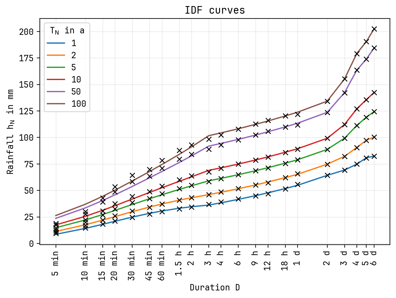
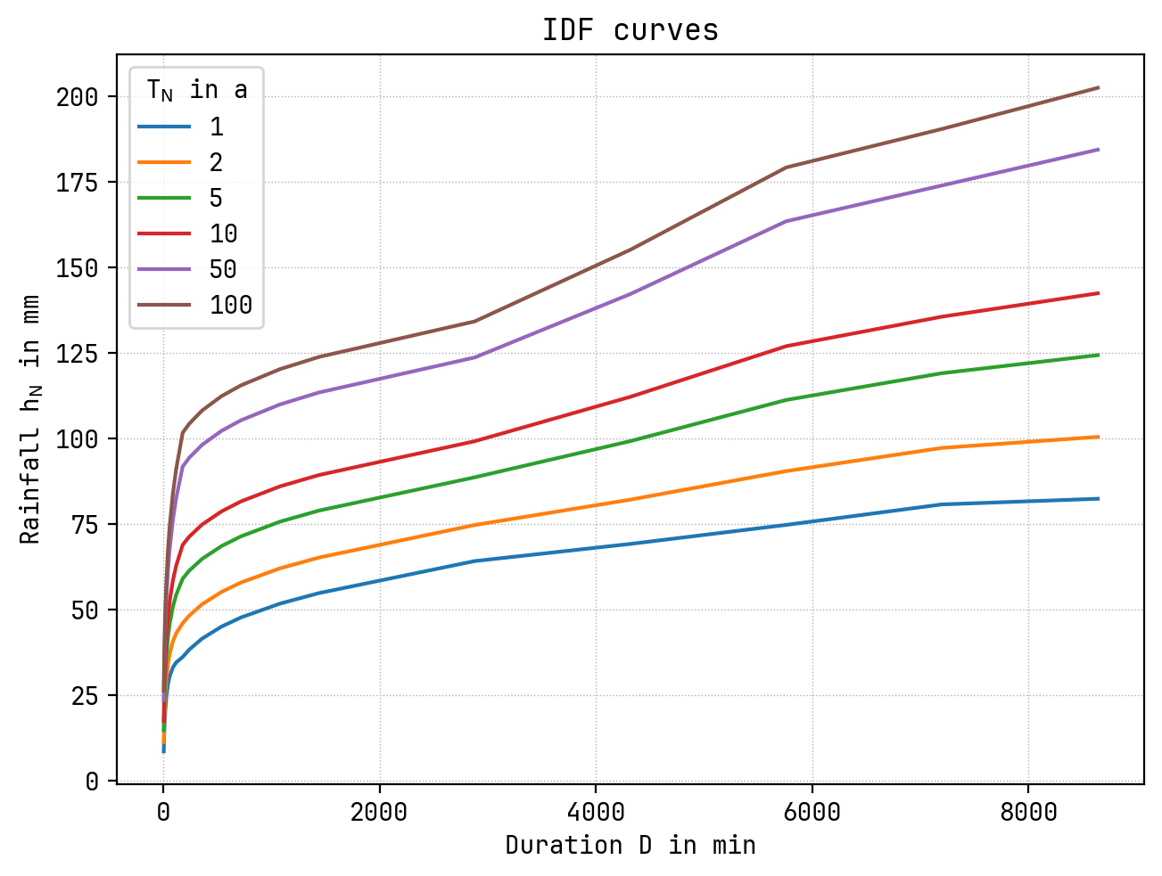
To create a color plot of the IDF curves:

[28]:

fig, ax = idf.curve_figure(color=True, add_interim=False)

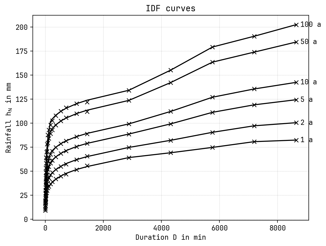
../_images/examples_example_python_api_42_0.png

To create a black/white plot of the IDF curves:

[29]:

fig, ax = idf.curve_figure(color=False, add_interim=True)

../_images/examples_example_python_api_44_0.png

[30]:

fig, ax = idf.curve_figure(color=True, add_interim=True, logx=True, duration_steps_ticks=True)

../_images/examples_example_python_api_45_0.png

Intensity Duration Frequency Analyse¶

Parameter¶

Calculations¶

Table of Contents

Previous topic

Next topic

This Page